4  Tutorial 4

4.1 Topics

1. K-means clustering

2. Hierarchical clustering

4.2 K-Means Clustering

The k-means clustering method is an unsupervised machine learning technique used to identify clusters of data objects in a dataset. There are many different types of clustering methods, but k-means is one of the oldest and most approachable. These traits make implementing k-means clustering in Python reasonably straightforward, even for novice programmers and data scientists.

The k-means algorithm searches for a pre-determined number of clusters within an unlabeled multidimensional dataset. It accomplishes this using a simple conception of what the optimal clustering looks like:

The “cluster center” is the arithmetic mean of all the points belonging to the cluster. Each point is closer to its own cluster center than to other cluster centers.

https://jakevdp.github.io/PythonDataScienceHandbook/05.11-k-means.html

https://realpython.com/k-means-clustering-python/#:~:text=The%20k%2Dmeans%20clustering%20method,data%20objects%20in%20a%20dataset.&text=You’ll%20walk%20through%20an,the%20data%20to%20evaluating%20results.

4.3 Example

# import packages
import matplotlib.pyplot as plt
import seaborn as sns
import numpy as np
from sklearn.datasets import make_blobs
from sklearn.cluster import KMeans
from sklearn.metrics import silhouette_score
from scipy.cluster.hierarchy import fcluster

4.3.1 Starting from the end

Before getting to the algorithm itself, let’s see what K-Means actually does

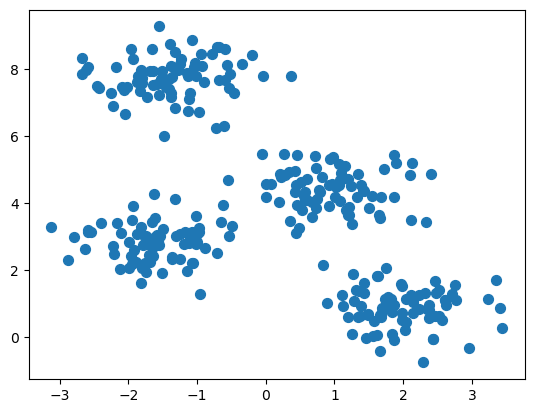
4.3.2 Create random data grouped in four “blobs”

X, y_true = make_blobs(n_samples=300, 
                       centers=4,
                       cluster_std=0.60, 
                       random_state=0)
plt.scatter(X[:, 0],
            X[:, 1],
            s=50);

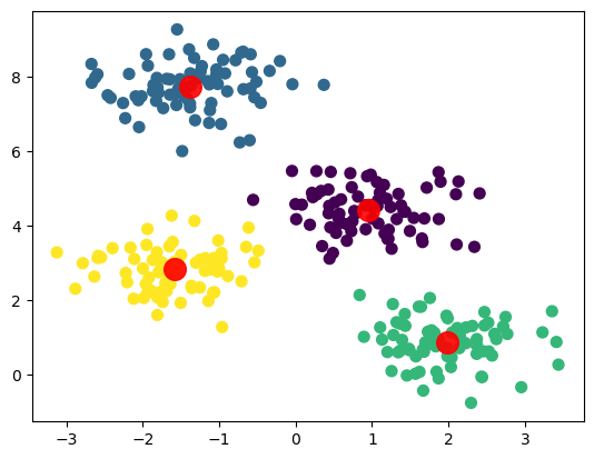
4.3.3 Calculate K-Means

kmeans = KMeans(n_clusters=4)
kmeans.fit(X)
clusters_kmeans = kmeans.predict(X)
clusters_kmeans

/opt/anaconda3/lib/python3.11/site-packages/sklearn/cluster/_kmeans.py:870: FutureWarning: The default value of `n_init` will change from 10 to 'auto' in 1.4. Set the value of `n_init` explicitly to suppress the warning
  warnings.warn(

array([2, 1, 0, 1, 2, 2, 3, 0, 1, 1, 3, 1, 0, 1, 2, 0, 0, 2, 3, 3, 2, 2,
       0, 3, 3, 0, 2, 0, 3, 0, 1, 1, 0, 1, 1, 1, 1, 1, 3, 2, 0, 3, 0, 0,
       3, 3, 1, 3, 1, 2, 3, 2, 1, 2, 2, 3, 1, 3, 1, 2, 1, 0, 1, 3, 3, 3,
       1, 2, 1, 3, 0, 3, 1, 3, 3, 1, 3, 0, 2, 1, 2, 0, 2, 2, 1, 0, 2, 0,
       1, 1, 0, 2, 1, 3, 3, 0, 2, 2, 0, 3, 1, 2, 1, 2, 0, 2, 2, 0, 1, 0,
       3, 3, 2, 1, 2, 0, 1, 2, 2, 0, 3, 2, 3, 2, 2, 2, 2, 3, 2, 3, 1, 3,
       3, 2, 1, 3, 3, 1, 0, 1, 1, 3, 0, 3, 0, 3, 1, 0, 1, 1, 1, 0, 1, 0,
       2, 3, 1, 3, 2, 0, 1, 0, 0, 2, 0, 3, 3, 0, 2, 0, 0, 1, 2, 0, 3, 1,
       2, 2, 0, 3, 2, 0, 3, 3, 0, 0, 0, 0, 2, 1, 0, 3, 0, 0, 3, 3, 3, 0,
       3, 1, 0, 3, 2, 3, 0, 1, 3, 1, 0, 1, 0, 3, 0, 0, 1, 3, 3, 2, 2, 0,
       1, 2, 2, 3, 2, 3, 0, 1, 1, 0, 0, 1, 0, 2, 3, 0, 2, 3, 1, 3, 2, 0,
       2, 1, 1, 1, 1, 3, 3, 1, 0, 3, 2, 0, 3, 3, 3, 2, 2, 1, 0, 0, 3, 2,
       1, 3, 0, 1, 0, 2, 2, 3, 3, 0, 2, 2, 2, 0, 1, 1, 2, 2, 0, 2, 2, 2,
       1, 3, 1, 0, 2, 2, 1, 1, 1, 2, 2, 0, 1, 3], dtype=int32)

len(clusters_kmeans)

300

4.3.4 Plot results

# blobs
plt.scatter(X[:, 0], 
            X[:, 1], 
            c=clusters_kmeans, 
            s=50, 
            cmap='viridis')

# center of blob
centers = kmeans.cluster_centers_
plt.scatter(centers[:, 0], 
            centers[:, 1], 
            c='red', 
            s=200, 
            alpha=0.9)

<matplotlib.collections.PathCollection at 0x125c68b90>

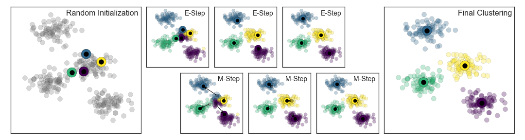
4.3.5 How does the algorithm work?

K-Means uses the Expectation-Maximization Algorithm

How does this work?

1. Guess some cluster centers
2. Repeat until converged
   • E-Step: assign points to the nearest cluster center
   • M-Step: set the cluster centers to the mean

The “E-step” or “Expectation step” involves updating our expectation of which cluster each point belongs to.

The “M-step” or “Maximization step” involves maximizing some fitness function that defines the location of the cluster centers. In this case, that maximization is accomplished by taking a simple mean of the data in each cluster.

%matplotlib inline
from IPython.display import Image
Image('image_1.png')

4.3.6 Visualisation

Here is a cool video for visualising the prosses of K-means clustering.

4.3.7 Choosing the right number of clusters

We’ll look at two methods for choosing the correct number of clusters.

The elbow method and the silhouette method. We can use these methods together. No need to pick just one.

The quality of the cluster assignments is determined by computing the sum of the squared error (SSE) after the centroids converge.

SSE is defined as the sum of the squared distance between centroid and each member of the cluster.

4.3.8 The elbow method

To perform the elbow method, run several k-means, increment k with each iteration, and record the SSE.

# loop over different numbers of clusters
kmeans_kwargs = {"init": "random",
                 "n_init": 10,
                 "max_iter": 300,
                 "random_state": 42,}

# A list holds the SSE values for each k
sse = []
for k in range(1, 11):
    kmeans = KMeans(n_clusters=k, **kmeans_kwargs)
    kmeans.fit(X)
    error = kmeans.inertia_
    sse.append(kmeans.inertia_)
    print(f"With {k} clusters the SSE was {error}")

With 1 clusters the SSE was 2812.137595303235
With 2 clusters the SSE was 1190.7823593643443
With 3 clusters the SSE was 546.8911504626299
With 4 clusters the SSE was 212.00599621083478
With 5 clusters the SSE was 188.77323556773723
With 6 clusters the SSE was 170.94840955438684
With 7 clusters the SSE was 154.8848618157605
With 8 clusters the SSE was 139.20927769246356
With 9 clusters the SSE was 126.56204002887225
With 10 clusters the SSE was 111.8591054874254

# plot the data
plt.plot(range(1, 11), sse)
plt.xticks(range(1, 11))
plt.xlabel("Number of Clusters")
plt.ylabel("SSE")
plt.show()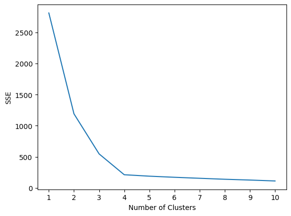

Determining the elbow point in the SSE curve isn’t always straightforward. If you’re having trouble choosing the elbow point of the curve, then you could use a Python package, kneed, to identify the elbow point programmatically.

4.3.9 The silhouette coefficient

The silhouette coefficient is a measure of cluster cohesion and separation. It quantifies how well a data point fits into its assigned cluster based on two factors: 1. How close the data point is to other points in the cluster 2. How far away the data point is from points in other clusters

Silhouette coefficient values range between -1 and 1. Larger numbers indicate that samples are closer to their clusters than they are to other clusters.

# A list holds the silhouette coefficients for each k
silhouette_coefficients = []

# Notice you start at 2 clusters for silhouette coefficient
for k in range(2, 11):
    kmeans = KMeans(n_clusters=k, **kmeans_kwargs)
    kmeans.fit(X)
    score = silhouette_score(X, kmeans.labels_)
    silhouette_coefficients.append(score)
    print(f"With {k} clusters the score was {score}")

With 2 clusters the score was 0.5426422297358303
With 3 clusters the score was 0.5890390393551768
With 4 clusters the score was 0.6819938690643478
With 5 clusters the score was 0.5923875148758644
With 6 clusters the score was 0.49563409602576686
With 7 clusters the score was 0.4277257665723784
With 8 clusters the score was 0.32252064195197455
With 9 clusters the score was 0.3335178002757919
With 10 clusters the score was 0.34598612018426733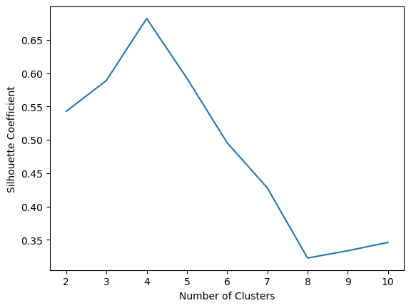

plt.plot(range(2, 11), silhouette_coefficients)
plt.xticks(range(2, 11))
plt.xlabel("Number of Clusters")
plt.ylabel("Silhouette Coefficient")
plt.show()

5 Hierarchical Clustering

Hierarchical clustering is a type of unsupervised machine learning algorithm used to cluster unlabeled data points. Hierarchical clustering groups together data points with similar characteristics.

There are two types of hierarchical clustering: agglomerative and divisive. * Agglomerative: data points are clustered using a bottom-up approach starting with individual data points * Divisive: all the data points are treated as one big cluster and the clustering process involves dividing the one big cluster into several small clusters.

Today, we’ll focus on agglomerative clustering.

https://scikit-learn.org/stable/auto_examples/cluster/plot_agglomerative_dendrogram.html
https://stackabuse.com/hierarchical-clustering-with-python-and-scikit-learn
https://joernhees.de/blog/2015/08/26/scipy-hierarchical-clustering-and-dendrogram-tutorial/

5.0.1 Steps to perform agglomerative clustering

1. Treat each data point as its own cluster. The number of clusters at the start will be K, where K is the number of data points.
2. Reduce the data to K-1 clusters by joining the two closest clusters (data points).
3. Reduce the data to K-2 clusters by again joining the two closest clusters.
4. Repeat this process until one big cluster is formed.
5. Develop dendograms to analyze the clusters.

5.0.2 Visualisation

Here is a video for visualising the prosses of hierarchical clustering.

5.0.3 Worked Example

# import packages 
import numpy as np
import pandas as pd
from matplotlib import pyplot as plt
import scipy.cluster.hierarchy as shc
from sklearn.cluster import AgglomerativeClustering

# make up data
points = np.array([[5,3],
                   [10,15],
                   [15,12],
                   [24,10],
                   [30,30],
                   [85,70],
                   [71,80],
                   [60,78],
                   [70,55],
                   [80,91],])

# plot the data
labels = range(1, 11)
plt.figure()
plt.scatter(points[:,0], 
            points[:,1], 
            label='True Position')

for label, x, y in zip(labels, points[:, 0], points[:, 1]):
    plt.annotate(label,
                 xy=(x, y), 
                 xytext=(-3, 3),
                 textcoords='offset points', 
                 ha='right', 
                 va='bottom')

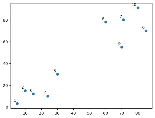
5.0.4 Do you see any “clusters”?

linked = shc.linkage(points, 'single')

labelList = range(1, 11)

fig = plt.figure()
shc.dendrogram(linked,
               orientation='top',
               labels=labelList,
               distance_sort='descending',
               show_leaf_counts=True)
plt.xlabel('Points')
plt.ylabel('Euclidean Distance')
plt.axhline(y= 30, c='purple', ls = '--')

<matplotlib.lines.Line2D at 0x127e6b710>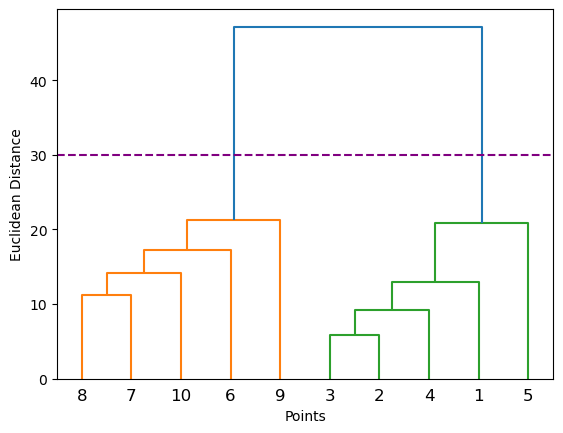

5.0.4.1 Where is the longest distance without a horizontal line?

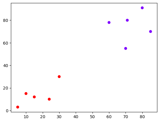
# create actual clusters
cluster = AgglomerativeClustering(n_clusters=2,
                                  affinity='euclidean', 
                                  linkage='ward')
cluster.fit_predict(points)

/opt/anaconda3/lib/python3.11/site-packages/sklearn/cluster/_agglomerative.py:983: FutureWarning: Attribute `affinity` was deprecated in version 1.2 and will be removed in 1.4. Use `metric` instead
  warnings.warn(

array([1, 1, 1, 1, 1, 0, 0, 0, 0, 0])

5.0.4.2 The output array shows us which cluster each point is in

# plot the original data with the clusters
plt.scatter(points[:,0], points[:,1], 
            c=cluster.labels_, 
            cmap='rainbow')

<matplotlib.collections.PathCollection at 0x127dfef90>

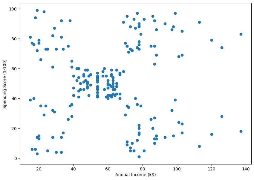
5.0.5 Example 2 – Real Data

download .csv here

# import data
customer_data = pd.read_csv('shopping-data.csv')
customer_data.head()

	CustomerID	Genre	Age	Annual Income (k$)	Spending Score (1-100)
0	1	Male	19	15	39
1	2	Male	21	15	81
2	3	Female	20	16	6
3	4	Female	23	16	77
4	5	Female	31	17	40

# isolate data from annual income and spending score columns
data = customer_data.iloc[:, 3:5].values
plt.figure(figsize=(10, 7))
plt.scatter(data[:,0], data[:,1])
plt.xlabel('Annual Income (k$)')
plt.ylabel('Spending Score (1-100)')

Text(0, 0.5, 'Spending Score (1-100)')

# examine dendogram
plt.figure()
plt.title("Customer Dendograms")
plt.xlabel('Points')
plt.ylabel('Euclidean Distance')
dend = shc.dendrogram(shc.linkage(data, method='ward'))

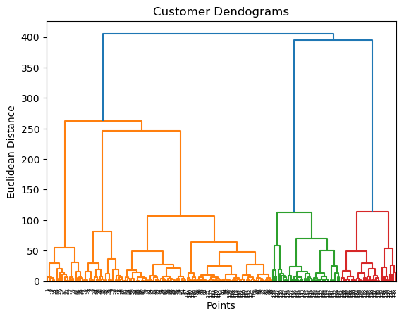
5.0.6 Finding the right number of clusters

5.0.6.1 Method 1: visualization

Where is the longest distance without a horizontal line?

Z = shc.linkage(data, method='ward')

plt.figure()
plt.title("Customer Dendograms")
plt.xlabel('Points')
plt.ylabel('Euclidean Distance')
dend = shc.dendrogram(Z)
plt.axhline(y= 200, c='purple', ls = '--')

<matplotlib.lines.Line2D at 0x128518b50>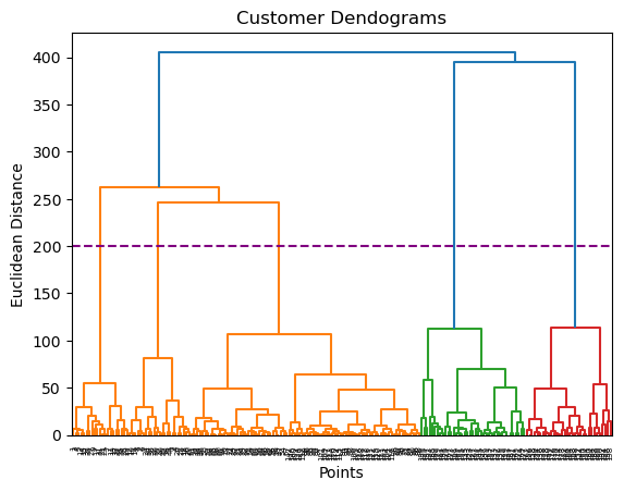

# create clusters
cluster = AgglomerativeClustering(n_clusters=5, affinity='euclidean', linkage='ward')
cluster.fit_predict(data)

/opt/anaconda3/lib/python3.11/site-packages/sklearn/cluster/_agglomerative.py:983: FutureWarning: Attribute `affinity` was deprecated in version 1.2 and will be removed in 1.4. Use `metric` instead
  warnings.warn(

array([4, 3, 4, 3, 4, 3, 4, 3, 4, 3, 4, 3, 4, 3, 4, 3, 4, 3, 4, 3, 4, 3,
       4, 3, 4, 3, 4, 3, 4, 3, 4, 3, 4, 3, 4, 3, 4, 3, 4, 3, 4, 3, 4, 1,
       4, 1, 1, 1, 1, 1, 1, 1, 1, 1, 1, 1, 1, 1, 1, 1, 1, 1, 1, 1, 1, 1,
       1, 1, 1, 1, 1, 1, 1, 1, 1, 1, 1, 1, 1, 1, 1, 1, 1, 1, 1, 1, 1, 1,
       1, 1, 1, 1, 1, 1, 1, 1, 1, 1, 1, 1, 1, 1, 1, 1, 1, 1, 1, 1, 1, 1,
       1, 1, 1, 1, 1, 1, 1, 1, 1, 1, 1, 1, 1, 2, 1, 2, 1, 2, 0, 2, 0, 2,
       1, 2, 0, 2, 0, 2, 0, 2, 0, 2, 1, 2, 0, 2, 1, 2, 0, 2, 0, 2, 0, 2,
       0, 2, 0, 2, 0, 2, 1, 2, 0, 2, 0, 2, 0, 2, 0, 2, 0, 2, 0, 2, 0, 2,
       0, 2, 0, 2, 0, 2, 0, 2, 0, 2, 0, 2, 0, 2, 0, 2, 0, 2, 0, 2, 0, 2,
       0, 2])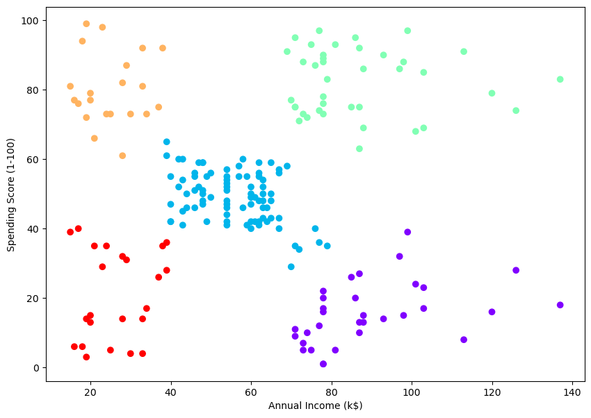

# look at the clusters
plt.figure(figsize=(10, 7))
plt.scatter(data[:,0], data[:,1], c=cluster.labels_, cmap='rainbow')
plt.xlabel('Annual Income (k$)')
plt.ylabel('Spending Score (1-100)')

Text(0, 0.5, 'Spending Score (1-100)')

5.0.6.2 Method 2: threshold

we don’t need to count the number of clusters, it’s enough to give the threshold value.

# Set the threshold value where you want to cut the dendrogram
threshold_value = 150  # Adjust this value as needed

# Assuming 'data' is your dataset
Z = shc.linkage(data, method='ward')

# Plot the dendrogram
plt.figure(figsize=(10, 7))
dend = shc.dendrogram(Z)
plt.axhline(y=threshold_value, color='r', linestyle='--')
plt.show()

# Get the cluster labels
clusters = fcluster(Z, threshold_value, criterion='distance')

# Print the number of clusters
num_clusters = len(set(clusters))
print(f'The number of clusters is: {num_clusters}')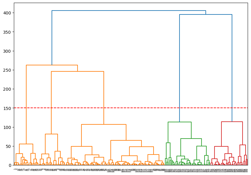

The number of clusters is: 5

5.0.6.3 Method 3: silhouette

# Assuming 'data' is your dataset and 'Z' is the linkage matrix
range_n_clusters = list(range(2, 101))
silhouette_scores = []

for n_clusters in range_n_clusters:
    cluster_labels = fcluster(Z, n_clusters, criterion='maxclust')
    silhouette_avg = silhouette_score(data, cluster_labels)
    silhouette_scores.append(silhouette_avg)
    # print(f"For n_clusters = {n_clusters}, the silhouette score is: {silhouette_avg}")

# Plot the silhouette scores
fig, ax = plt.subplots()
ax.plot(range_n_clusters, silhouette_scores, marker='o')
ax.set_title('Silhouette Scores for Various Numbers of Clusters')
ax.set_xlabel('Number of Clusters')
ax.set_ylabel('Silhouette Score')
plt.show()

print(f'Max silhouette score at {silhouette_scores.index(max(silhouette_scores))+2} clusters')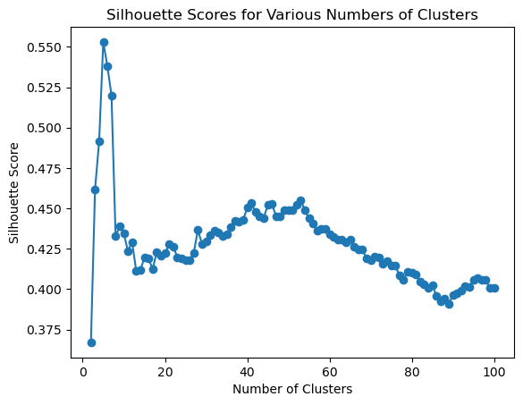

Max silhouette score at 5 clusters

6 Play Time

Use the dataset cluster_play_data.csv to play with the clustering method we learned. download .csv here
First step hint - try to find out on what columns to preform the clustering.

Answer part 1

# import data

# # uncomment below:
# play = pd.read_csv('cluster_play_data.csv')
# play.head()

Answer part 2

# # uncomment below:
# sns.pairplot(play)

Answer part 3

# # uncomment below:
# # examine dendogram
# # isolate data from annual income and spending score columns
# # data = customer_data.iloc[:, 3:5].values
# data = play[['A','C']].values
# plt.figure()
# plt.title("Customer Dendograms")
# plt.xlabel('Points')
# plt.ylabel('Euclidean Distance')
# dend = shc.dendrogram(shc.linkage(data, method='ward'))

Answer part 4

# # uncomment below:
# # create clusters
# cluster = AgglomerativeClustering(n_clusters=6, affinity='euclidean', linkage='ward')
# cluster.fit_predict(data)

# # look at the clusters
# plt.figure(figsize=(10, 7))
# plt.scatter(data[:,0], data[:,1], c=cluster.labels_, cmap='rainbow')
# plt.xlabel('Annual Income (k$)')
# plt.ylabel('Spending Score (1-100)')