6 Tutorial 6

6.1 Topics

Hypothesis testing using permutations
t-test with the scipy.stats library

6.2 Hypothesis testing

A statistical hypothesis test is a method of statistical inference used to decide whether the data at hand sufficiently support a particular hypothesis.

https://en.wikipedia.org/wiki/Statistical_hypothesis_testing

6.3 Permutation tests

A permutation test (also called a randomization test, re-randomization test, or an exact test) is a type of statistical significance test in which the distribution of the test statistic under the null hypothesis is obtained by calculating all possible values of the test statistic under all possible rearrangements of the observed data points

https://en.wikipedia.org/wiki/Resampling_(statistics)#Permutation_tests

To illustrate the basic idea of a permutation test, suppose we collect random variables X_A and X_B for each individual from two groups A and B whose sample means are \bar{x}_{A} and \bar{x}_{B}, and that we want to know whether X_A and X_B come from the same distribution. Let n_{A} and n_{B} be the sample size collected from each group. The permutation test is designed to determine whether the observed difference between the sample means is large enough to reject, at some significance level, the null hypothesis H_{0} that the data drawn from A is from the same distribution as the data drawn from B.

The test proceeds as follows. First, the difference in means between the two samples is calculated: this is the observed value of the test statistic,T_\text{obs}.

Next, the observations of groups A and B are pooled, and the difference in sample means is calculated and recorded for every possible way of dividing the pooled values into two groups of size n_{A} and n_{B} (i.e., for every permutation of the group labels A and B). The set of these calculated differences is the exact distribution of possible differences (for this sample) under the null hypothesis that group labels are exchangeable (i.e., are randomly assigned).

The one-sided p-value of the test is calculated as the proportion of sampled permutations where the difference in means was greater than or equal to T_\text{obs}. The two-sided p-value of the test is calculated as the proportion of sampled permutations where the [[absolute difference]] was greater than or equal to |T_\text{obs}|.

Alternatively, if the only purpose of the test is to reject or not reject the null hypothesis, one could sort the recorded differences, and then observe if T_\text{obs} is contained within the middle (1 - \alpha) \times 100% of them, for some significance level \alpha. If it is not, we reject the hypothesis of identical probability curves at the \alpha\times100\% significance level.

6.3.1 The Iris dataset

The data set consists of 50 samples from each of three species of Iris (Iris setosa, Iris virginica and Iris versicolor). Four features were measured from each sample: the length and the width of the sepals and petals, in centimeters.

6.4 Our Null Hypothesis

There is no difference between mean sepal length for Iris virginca and Iris versicolor.

# import packages
import numpy as np
from sklearn import datasets
import pandas as pd

iris = datasets.load_iris()
df= pd.DataFrame(data= np.c_[iris['data'], iris['target']],
                 columns= iris['feature_names'] + ['target'])
df['species'] = pd.Categorical.from_codes(iris.target, iris.target_names)

df.head(10)

	sepal length (cm)	sepal width (cm)	petal length (cm)	petal width (cm)	species
0	5.1	3.5	1.4	0.2	setosa
1	4.9	3.0	1.4	0.2	setosa
2	4.7	3.2	1.3	0.2	setosa
3	4.6	3.1	1.5	0.2	setosa
4	5.0	3.6	1.4	0.2	setosa
5	5.4	3.9	1.7	0.4	setosa
6	4.6	3.4	1.4	0.3	setosa
7	5.0	3.4	1.5	0.2	setosa
8	4.4	2.9	1.4	0.2	setosa
9	4.9	3.1	1.5	0.1	setosa

We’ll use a permutation test to compare the mean sepal length for Iris virginca and Iris versicolor. We start by comparing the actual mean sepal length for the species we’re intrested in.

# group by species
by_species = df.groupby("species")
by_species.head(10)

/var/folders/wn/2bz1970d2w5182zy7h96yfcc0000gn/T/ipykernel_39706/2135608631.py:2: FutureWarning: The default of observed=False is deprecated and will be changed to True in a future version of pandas. Pass observed=False to retain current behavior or observed=True to adopt the future default and silence this warning.
  by_species = df.groupby("species")

	sepal length (cm)	sepal width (cm)	petal length (cm)	petal width (cm)	target	species
0	5.1	3.5	1.4	0.2	0.0	setosa
1	4.9	3.0	1.4	0.2	0.0	setosa
2	4.7	3.2	1.3	0.2	0.0	setosa
3	4.6	3.1	1.5	0.2	0.0	setosa
4	5.0	3.6	1.4	0.2	0.0	setosa
5	5.4	3.9	1.7	0.4	0.0	setosa
6	4.6	3.4	1.4	0.3	0.0	setosa
7	5.0	3.4	1.5	0.2	0.0	setosa
8	4.4	2.9	1.4	0.2	0.0	setosa
9	4.9	3.1	1.5	0.1	0.0	setosa
50	7.0	3.2	4.7	1.4	1.0	versicolor
51	6.4	3.2	4.5	1.5	1.0	versicolor
52	6.9	3.1	4.9	1.5	1.0	versicolor
53	5.5	2.3	4.0	1.3	1.0	versicolor
54	6.5	2.8	4.6	1.5	1.0	versicolor
55	5.7	2.8	4.5	1.3	1.0	versicolor
56	6.3	3.3	4.7	1.6	1.0	versicolor
57	4.9	2.4	3.3	1.0	1.0	versicolor
58	6.6	2.9	4.6	1.3	1.0	versicolor
59	5.2	2.7	3.9	1.4	1.0	versicolor
100	6.3	3.3	6.0	2.5	2.0	virginica
101	5.8	2.7	5.1	1.9	2.0	virginica
102	7.1	3.0	5.9	2.1	2.0	virginica
103	6.3	2.9	5.6	1.8	2.0	virginica
104	6.5	3.0	5.8	2.2	2.0	virginica
105	7.6	3.0	6.6	2.1	2.0	virginica
106	4.9	2.5	4.5	1.7	2.0	virginica
107	7.3	2.9	6.3	1.8	2.0	virginica
108	6.7	2.5	5.8	1.8	2.0	virginica
109	7.2	3.6	6.1	2.5	2.0	virginica

Seperate out the species we’re interested in

virginica = by_species.get_group("virginica")
versicolor = by_species.get_group("versicolor")

work with only 10 rows of each species (this is done to make things more interesting because the more rows we look at the more significant result we will get in the end)

n_rows = 10  # number of rows to keep should be less than 50
virginica = virginica[0:n_rows]
versicolor = versicolor[0:n_rows]

Concatenate the two species into one data frame

data = pd.concat([virginica, versicolor])
data

	sepal length (cm)	sepal width (cm)	petal length (cm)	petal width (cm)	target	species
100	6.3	3.3	6.0	2.5	2.0	virginica
101	5.8	2.7	5.1	1.9	2.0	virginica
102	7.1	3.0	5.9	2.1	2.0	virginica
103	6.3	2.9	5.6	1.8	2.0	virginica
104	6.5	3.0	5.8	2.2	2.0	virginica
105	7.6	3.0	6.6	2.1	2.0	virginica
106	4.9	2.5	4.5	1.7	2.0	virginica
107	7.3	2.9	6.3	1.8	2.0	virginica
108	6.7	2.5	5.8	1.8	2.0	virginica
109	7.2	3.6	6.1	2.5	2.0	virginica
50	7.0	3.2	4.7	1.4	1.0	versicolor
51	6.4	3.2	4.5	1.5	1.0	versicolor
52	6.9	3.1	4.9	1.5	1.0	versicolor
53	5.5	2.3	4.0	1.3	1.0	versicolor
54	6.5	2.8	4.6	1.5	1.0	versicolor
55	5.7	2.8	4.5	1.3	1.0	versicolor
56	6.3	3.3	4.7	1.6	1.0	versicolor
57	4.9	2.4	3.3	1.0	1.0	versicolor
58	6.6	2.9	4.6	1.3	1.0	versicolor
59	5.2	2.7	3.9	1.4	1.0	versicolor

Get the actual mean sepal length for each

grouped = data.groupby("species", observed=True)['sepal length (cm)'].mean()
print(f'THe mean of sepal length for virginica is {grouped["virginica"]}')
print(f'THe mean of sepal length for versicolor is {grouped["versicolor"]}')

THe mean of sepal length for virginica is 6.57
THe mean of sepal length for versicolor is 6.1

abs_dif = np.abs(grouped["virginica"] - grouped["versicolor"])
print(f'The difference between the means is {abs_dif}')

The difference between the means is 0.47000000000000064

data['species_shuffled'] = data['species'].sample(frac=1, replace=False).values
data

	sepal length (cm)	sepal width (cm)	petal length (cm)	petal width (cm)	target	species	species_shuffled
100	6.3	3.3	6.0	2.5	2.0	virginica	virginica
101	5.8	2.7	5.1	1.9	2.0	virginica	versicolor
102	7.1	3.0	5.9	2.1	2.0	virginica	versicolor
103	6.3	2.9	5.6	1.8	2.0	virginica	virginica
104	6.5	3.0	5.8	2.2	2.0	virginica	versicolor
105	7.6	3.0	6.6	2.1	2.0	virginica	versicolor
106	4.9	2.5	4.5	1.7	2.0	virginica	versicolor
107	7.3	2.9	6.3	1.8	2.0	virginica	versicolor
108	6.7	2.5	5.8	1.8	2.0	virginica	virginica
109	7.2	3.6	6.1	2.5	2.0	virginica	virginica
50	7.0	3.2	4.7	1.4	1.0	versicolor	versicolor
51	6.4	3.2	4.5	1.5	1.0	versicolor	virginica
52	6.9	3.1	4.9	1.5	1.0	versicolor	virginica
53	5.5	2.3	4.0	1.3	1.0	versicolor	versicolor
54	6.5	2.8	4.6	1.5	1.0	versicolor	virginica
55	5.7	2.8	4.5	1.3	1.0	versicolor	virginica
56	6.3	3.3	4.7	1.6	1.0	versicolor	versicolor
57	4.9	2.4	3.3	1.0	1.0	versicolor	virginica
58	6.6	2.9	4.6	1.3	1.0	versicolor	versicolor
59	5.2	2.7	3.9	1.4	1.0	versicolor	virginica

data['species_shuffled'] = data['species'].sample(frac=1, replace=False).values
grouped = data.groupby("species_shuffled", observed=True)['sepal length (cm)'].mean()
print(f'The mean of sepal length for virginica is {grouped["virginica"]}')
print(f'The mean of sepal length for versicolor is {grouped["versicolor"]}')

sampled_diff = np.abs(grouped["virginica"] - grouped["versicolor"])
print(f'The difference between the means is {sampled_diff}')

The mean of sepal length for virginica is 6.58
The mean of sepal length for versicolor is 6.09
The difference between the means is 0.4900000000000002

runs = 1000
diffs = np.zeros(runs)
for ii in range(runs):
    data['species_shuffled'] = data['species'].sample(frac=1, replace=False).values
    grouped = data.groupby("species_shuffled", observed=True)['sepal length (cm)'].mean()
    diffs[ii]= np.abs(grouped["virginica"] - grouped["versicolor"])

# compute our p-value
larger = np.where(diffs>=abs_dif, 1, 0)
p_val = np.sum(larger)/runs
print(f'The p-value is {p_val}')
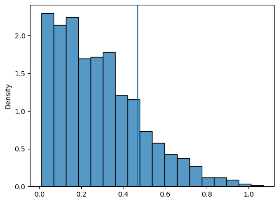
np.sum(larger)

The p-value is 0.181

6.4.1 Let’s look at it visually

import seaborn as sns
ax = sns.histplot(diffs, stat='density')
ax.axvline(abs_dif)

<matplotlib.lines.Line2D at 0x128ad8bd0>

7 3. Using `scipy.stats` tests

We can compare the results above to a t-test using the scipy.stats library

7.0.1 The scipy.stats library

This module contains a large number of probability distributions, summary and frequency statistics, correlation functions and statistical tests, masked statistics, kernel density estimation, quasi-Monte Carlo functionality, and more.

https://docs.scipy.org/doc/scipy/reference/stats.html

import scipy.stats as stats

stats.ttest_ind(virginica['sepal length (cm)'], versicolor['sepal length (cm)'])

TtestResult(statistic=1.3707421122118832, pvalue=0.18730715303330478, df=18.0)