6 Bootstrapping and Confidence Intervals
TA 5
6.1 Topics
- Standard error vs. Standard deviation
- Boostrapping
- Confidence Intervals
6.2 Standard error vs. standard deviation
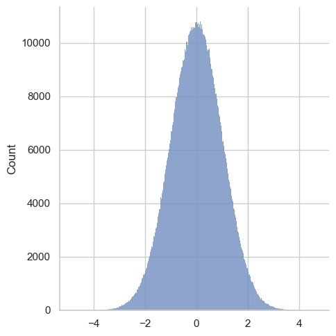
Let’s define a “population” of size 1,000,000. Each member of the population will be a number from the standard normal distribution. We will be using the numpy function randn
What’s the population’s mean and standard deviation?
mean_value = population.mean()
std = population.std()
print(f"The mean value is {mean_value} and the standard deviation is {std}")
The mean value is -0.0015997564542563718 and the standard deviation is 1.000188036804731What does the distribution of the population look like?
If this were the real world, sampling 1,000,000 people would be difficult. Let’s say that our budget allowed us to sample only 100 people at a time. How can we simulate that?
What’s the sample’s mean and standard deviation?
mean_100 = sample_100.mean()
std_100 = sample_100.std()
print(f"The mean value is {mean_100}\nThe standard deviation is {std_100}")
The mean value is -0.1753180501180135
The standard deviation is 1.1706030198688049Notice that our sample’s mean value is pretty different from that of the population. What if we take a bigger sample size?
sample_size = 1000
sample_1000 = np.random.choice(population, sample_size)
mean_1000 = sample_1000.mean()
std_1000 = sample_1000.std()
print(f"The mean value is {mean_1000}\nThe standard deviation is {std_1000}")
The mean value is -0.008352574043024205
The standard deviation is 1.003117759041072Or smaller…
sample_size = 5
sample_5 = np.random.choice(population, sample_size)
mean_5 = sample_5.mean()
std_5 = sample_5.std()
print(f"The mean value is {mean_5}\nThe standard deviation is {std_5}")
The mean value is 0.03172109602313291
The standard deviation is 0.758566765992809The standard error of the mean (SEM) measures the precision of the estimate of the sample mean. We can use the formula:
\text{SEM} = \frac{\sigma}{\sqrt{n}}
- \sigma = the standard deviation of the sample
- n = the sample size
Now we can compare our standard errors using the different sample sizes.
se_5 = std_5/np.sqrt(5)
se_100 = std_100/np.sqrt(100)
se_1000 = std_1000/np.sqrt(1000)

print(f"The SEM when the sample size was 5 was {se_5}")
print(f"The SEM when the sample size was 100 was {se_100}")
print(f"The SEM when the sample size was 1000 was {se_1000}")
The SEM when the sample size was 5 was 0.3392413708464193
The SEM when the sample size was 100 was 0.11706030198688049
The SEM when the sample size was 1000 was 0.031721368799337497 Bootstrapping
Bootstrapping is a statistical method that involves repeatedly resampling a dataset with replacement to estimate the distribution of a statistic. This technique allows for the assessment of the accuracy and variability of sample estimates, such as the mean or standard deviation, without making strict assumptions about the underlying population distribution. By generating many resampled datasets (called bootstrap samples) and calculating the statistic of interest for each sample, bootstrapping provides an empirical approximation of the sampling distribution. This method is particularly useful when dealing with small samples or when traditional parametric assumptions cannot be applied.
Let’s create a numpy array to represent heights of females at the Faculta
np.random.seed(42)
mean = 162.2
std = 5.5
sample_size = 1000
heights = np.random.normal(loc=mean,
                           scale=std,
                           size=sample_size)

# sample mean
mean_value = heights.mean()

# population standard deviation
std = heights.std()

print(f"The population's mean value is {mean_value}\nThe standard deviation is {std}")
The population's mean value is 162.30632630702277
The standard deviation is 5.382994142610448Now we can construct a simulated sampling distribution
# now we can find the standard deviation of the means
se_mean_height_bootstrap = sample_means.std()
print(f"The standard error of the mean calculated using bootstrapping is: {se_mean_height_bootstrap:.3f}")
The standard error of the mean calculated using bootstrapping is: 0.175Reminder, for the mean, it is also possible to estimate the Standard Error (SE) of the mean by dividing the standard deviation (STD) of the values by the square root of the sample size. The formula for the Standard Error of the Mean (SEM) is:
\text{SEM} = \frac{\sigma}{\sqrt{n}}
where \sigma is the standard deviation of the sample, and n is the sample size.
For other statistics, such as the median, there is no such analytical formula. The utility of the bootstrap method lies in its ability to estimate the SE of these other statistics. By repeatedly resampling the data with replacement and calculating the statistic of interest for each resample, bootstrapping provides an empirical distribution of the statistic. From this distribution, we can estimate the SE and other measures of variability.
se_mean_height_analytical = heights.std()/np.sqrt(sample_size)
print(f"The standard error of the mean calculated using the analytical formula is: {se_mean_height_analytical:.3f}")
The standard error of the mean calculated using the analytical formula is: 0.1707.1 Confidence Intervals
We can also compute the confidence interval for our estimate of the mean. Let’s say we want the 90 percent confidence interval.
7.2 Can you bootsrap confidence interval for the median?
Answer
# make a bootstrapped population of the median
boot_straps = 500
sample_size
sample_medians = np.zeros(boot_straps)
for ii in range(boot_straps):
    sample = np.random.choice(heights,
                              size=sample_size,
                              replace=True)
    sample_medians[ii]= np.median(sample)

# compute CI for the bootstrapped population of the median
conf_level = 0.9
low_bound = (1-conf_level)/2
up_bound = (1+conf_level)/2
CI = (np.quantile(sample_medians, low_bound),
      np.quantile(sample_medians, up_bound))

# # uncomment below:
# print(f"The lower bound of the confidence interval is: {CI[0]}")
# print(f"The upper bound of the confidence interval is: {CI[1]}")