10 Logistic regression

In statistics, the logistic model (or logit model) is used to model the probability of a certain class or event existing such as pass/fail, win/lose, alive/dead or healthy/sick. This can be extended to model several classes of events such as determining whether an image contains a cat, dog, lion, etc. Each object being detected in the image would be assigned a probability between 0 and 1, with a sum of one.

https://en.wikipedia.org/wiki/Logistic_regression

10.1 What’s the difference between linear regression and logistic regression?

Logistic regression analysis is used to examine the association of (categorical or continuous) independent variable(s) with one dichotomous dependent variable. This is in contrast to linear regression analysis in which the dependent variable is a continuous variable.

https://www.javatpoint.com/linear-regression-vs-logistic-regression-in-machine-learning

10.2 Logistic regression in Python

https://realpython.com/logistic-regression-python/

https://towardsdatascience.com/building-a-logistic-regression-in-python-step-by-step-becd4d56c9c8

10.3 Logistic regression: simple example

Import packages

import numpy as np
from sklearn.linear_model import LogisticRegression
from scipy.special import expit
import matplotlib.pyplot as plt
from sklearn.metrics import confusion_matrix
import seaborn as sns

Make up data

x = np.arange(10).reshape(-1, 1)
y = np.array([0, 0, 0, 0, 1, 1, 1, 1, 1, 1])

array([[0],
       [1],
       [2],
       [3],
       [4],
       [5],
       [6],
       [7],
       [8],
       [9]])

Note: we use reshape on x because when using the LogisticRegression function the x array must be two-dimensional.

Using reshape() with the arguments -1, 1 gives us as many rows as needed and one column.

fig, ax = plt.subplots()
ax.scatter(x, y, 
           color='black', 
           s=100, 
           label="actual data")
ax.set_xlabel("X")
ax.set_ylabel("Y")
ax.legend()

<matplotlib.legend.Legend at 0x128e72bd0>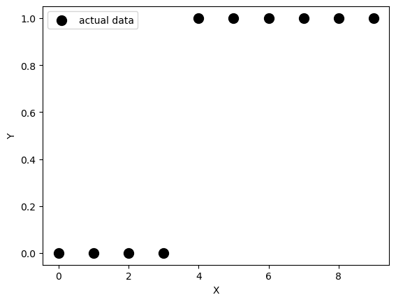

Create the model

model = LogisticRegression(solver='liblinear')

Train the model

model.fit(x, y)

LogisticRegression(solver='liblinear')

In a Jupyter environment, please rerun this cell to show the HTML representation or trust the notebook.
On GitHub, the HTML representation is unable to render, please try loading this page with nbviewer.org.

Alternatively, we can create and fit the model in just one step


model = LogisticRegression(solver='liblinear', random_state=0).fit(x, y)

Our potential y-values… not very surprising

model.classes_

array([0, 1])

The model’s intercept

model.intercept_

array([-1.04608067])

The model’s coefficient

model.coef_

array([[0.51491375]])

Evaluate the model

model.predict_proba(x)

array([[0.74002157, 0.25997843],
       [0.62975524, 0.37024476],
       [0.5040632 , 0.4959368 ],
       [0.37785549, 0.62214451],
       [0.26628093, 0.73371907],
       [0.17821501, 0.82178499],
       [0.11472079, 0.88527921],
       [0.07186982, 0.92813018],
       [0.04422513, 0.95577487],
       [0.02690569, 0.97309431]])

This returns the matrix of probabilities that the predicted output is equal to zero or one. The first column is the probability of the predicted output being zero, that is 1 - 𝑝(𝑥). The second column is the probability that the output is one, or 𝑝(𝑥).

You can get the actual predictions, based on the probability matrix and the values of 𝑝(𝑥), with .predict(). This function returns the predicted output values as a one-dimensional array.

model.predict(x)

array([0, 0, 0, 1, 1, 1, 1, 1, 1, 1])

Plot the results

fig, ax = plt.subplots()
ax.scatter(x, y,
           color='black', 
           s=100, 
           label="actual data")
ax.scatter(x, model.predict(x), 
           color='red', 
           label="predicted")
ax.legend()

<matplotlib.legend.Legend at 0x12b0c6010>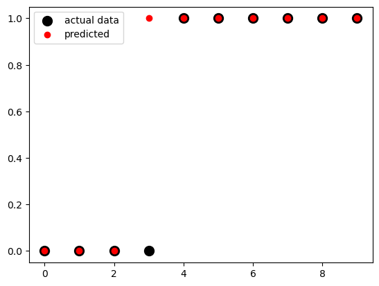

x_test = np.linspace(0, 10, 300).reshape(-1, 1)

fig, ax = plt.subplots()
ax.scatter(x, y, 
           color='black', 
           s=100, 
           label="actual data")
ax.scatter(x_test, 
           model.predict(x_test), 
           color='red', 
           label="predicted")
ax.legend()

<matplotlib.legend.Legend at 0x12b0b7c10>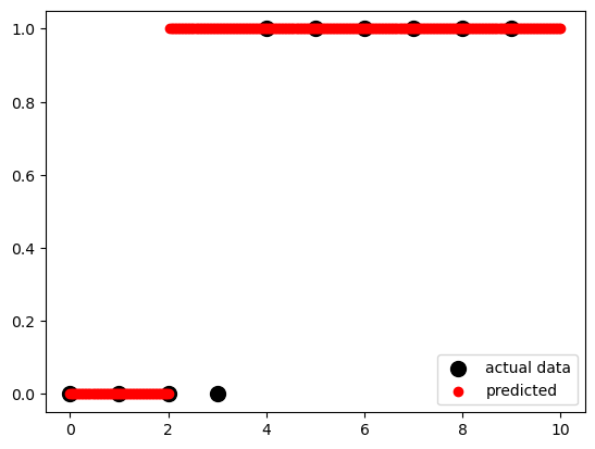

According to the logistic function:
### p=\frac{1}{1+e^{-(a+bx)}} * expit() This is a function from the SciPy library, specifically from the scipy.special module. It calculates the sigmoid function, which is defined as 1 / (1 + exp(-x)).
* .ravel() This function is called on the result of expit() to flatten or reshape the output as a 1-dimensional array. It converts a potentially multi-dimensional array into a contiguous flattened array.

sigmoid = expit(x_test * model.coef_ + model.intercept_).ravel()

fig, ax = plt.subplots()
ax.scatter(x, y, 
           color='black', 
           s=100, 
           label="actual data")
ax.scatter(x_test, 
           model.predict(x_test), 
           color='red', 
           label="predicted")
ax.plot(x_test, 
        sigmoid, 
        color='green', 
        linewidth=3, 
        label='logistic sigmoid')
ax.axhline(y=0.5, 
           color='black', 
           ls='--', 
           label='y = 0.5')
ax.legend()

<matplotlib.legend.Legend at 0x12b192990>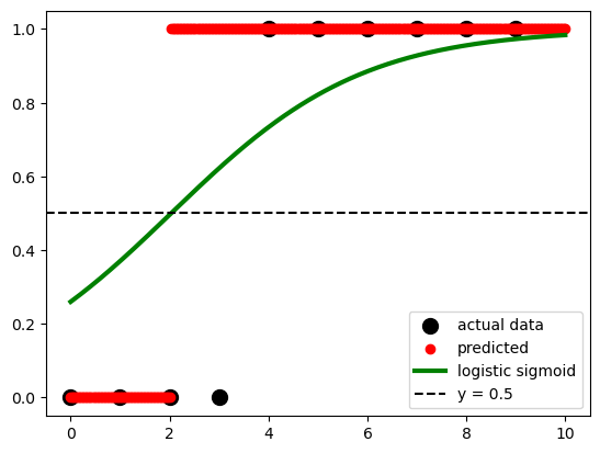

Get the model score


model.score(x, y)

0.9

# get the predicted values
y_pred = model.predict(x)

# create the confusion matrix
cm = confusion_matrix(y, y_pred)

# plot the confusion matrix using fig, ax method
fig, ax = plt.subplots()

sns.heatmap(cm, annot=True, cmap='Blues', ax=ax)
ax.set_xlabel('Predicted')
ax.set_ylabel('Actual')
ax.set_title('Confusion Matrix')

Text(0.5, 1.0, 'Confusion Matrix')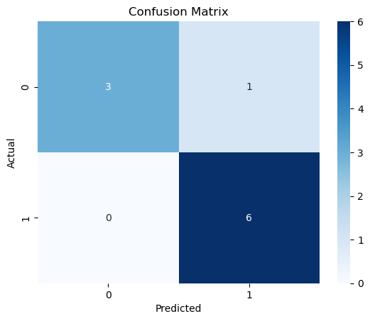

.score() takes the input and output as arguments and returns the ratio of the number of correct predictions to the number of observations.

10.3.1 We can also use the `StatsModels` packages, which provides some more statistical details

# import packages
import statsmodels.api as sm

# create data
x = np.arange(10).reshape(-1, 1)
y = np.array([0, 1, 0, 0, 1, 1, 1, 1, 1, 1])
x = sm.add_constant(x)

# create model
model = sm.Logit(y, x)

# fit model
result = model.fit()

# get results
result.params

Optimization terminated successfully.
         Current function value: 0.350471
         Iterations 7

array([-1.972805  ,  0.82240094])

print(result.summary())

                           Logit Regression Results                           
==============================================================================
Dep. Variable:                      y   No. Observations:                   10
Model:                          Logit   Df Residuals:                        8
Method:                           MLE   Df Model:                            1
Date:                Mon, 22 Jul 2024   Pseudo R-squ.:                  0.4263
Time:                        09:07:51   Log-Likelihood:                -3.5047
converged:                       True   LL-Null:                       -6.1086
Covariance Type:            nonrobust   LLR p-value:                   0.02248
==============================================================================
                 coef    std err          z      P>|z|      [0.025      0.975]
------------------------------------------------------------------------------
const         -1.9728      1.737     -1.136      0.256      -5.377       1.431
x1             0.8224      0.528      1.557      0.119      -0.213       1.858
==============================================================================

10.1 What’s the difference between linear regression and logistic regression?

10.2 Logistic regression in Python

10.3 Logistic regression: simple example

10.3.1 We can also use the StatsModels packages, which provides some more statistical details

10.3.1 We can also use the `StatsModels` packages, which provides some more statistical details