7 Tutorial 7

7.1 Dependence between variables

Correlation and regression
Linear regression – OLS

7.1.1 1. Correlation and Regression

Pearson’s coefficient measures linear correlation (r).
Spearman coefficient compares the ‘ranks’ of data.
NumPy, SciPy, and Pandas all have functions that can be used to calculate these coefficients.

7.1.2 Correlation in Numpy (Pearson’s r)

Required packages

import numpy as np
import seaborn as sns
import matplotlib.pyplot as plt

Let’s make up some numbers

mu, sigma = 0, 0.1 # mean and standard deviation
x = np.random.normal(mu, sigma, 50)
y = np.random.normal(mu, sigma, 50)
z = np.random.normal(mu, sigma, 50)

What does our data look like?

fig, ax = plt.subplots()
sns.scatterplot(x=x, y=y, ax=ax)
ax.set(xlabel='X', ylabel='Y')

[Text(0.5, 0, 'X'), Text(0, 0.5, 'Y')]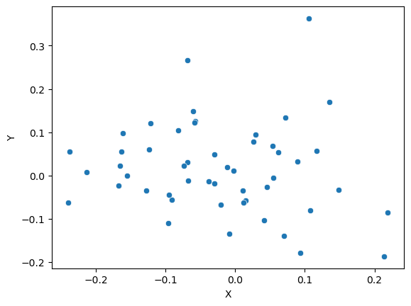

Use Numpy to get pearson’s correlation between x and y

np.corrcoef(x, y)

array([[ 1.        , -0.12455511],
       [-0.12455511,  1.        ]])

7.1.3 The result is a correlation matrix. Each cell in the table shows the correlation between two variables.

The values on the main diagonal of the correlation matrix (upper left and lower right) are equal to 1. These corresponds to the correlation coefficient for x and x and y and y, so they will always be equal to 1.
The values on the bottom left and top right show the pearson’s correlation coefficient for x and y.

We can do the same thing with more than two variables

np.corrcoef([x, y, z])

array([[ 1.        , -0.12455511,  0.03365426],
       [-0.12455511,  1.        , -0.14554429],
       [ 0.03365426, -0.14554429,  1.        ]])

7.2 Correlation in SciPy (Pearson and Spearman)

Import required packages

import scipy.stats

# pearson
scipy.stats.pearsonr(x, y)

PearsonRResult(statistic=-0.12455510674830719, pvalue=0.3887841983709771)

# spearman
scipy.stats.spearmanr(x, y)

SignificanceResult(statistic=-0.13661464585834332, pvalue=0.34413653070929573)

7.2.0.1 Note: these functions return both the correlation coefficient and the p-value

7.3 Correlation in Pandas

Time for some real data :)

7.3.1 Today’s dataset: Birthweight

This dataset contains information on new born babies and their parents.

https://www.sheffield.ac.uk/mash/statistics/datasets

Required packages

import pandas as pd

# import dataset
file = "./birthweight.csv"
df = pd.read_csv(file)

df.head()

	Length	Birthweight	Headcirc	Gestation	mage	mheight	mppwt	fage	fedyrs	fnocig	fheight	mage35
0	56	4.55	34	44	20	162	57	23	10	35	179	0
1	53	4.32	36	40	19	171	62	19	12	0	183	0
2	58	4.10	39	41	35	172	58	31	16	25	185	1
3	53	4.07	38	44	20	174	68	26	14	25	189	0
4	54	3.94	37	42	24	175	66	30	12	0	184	0

7.3.2 Is there any correlation between birthweight and head circumfrence?

# First, let's visualize the data
sns.scatterplot(x=df['Birthweight'], y=df['Headcirc'])

<Axes: xlabel='Birthweight', ylabel='Headcirc'>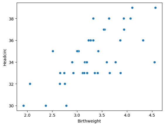

df['Birthweight'].corr(df['Headcirc'])

0.6846156184774087

7.3.3 There are lots of ways to calculate correlation in Pandas…

df['Birthweight'].corr(df['Headcirc'],
                       method='pearson')

0.6846156184774087

df['Birthweight'].corr(df['Headcirc'],
                       method='spearman')

0.6772599775176383

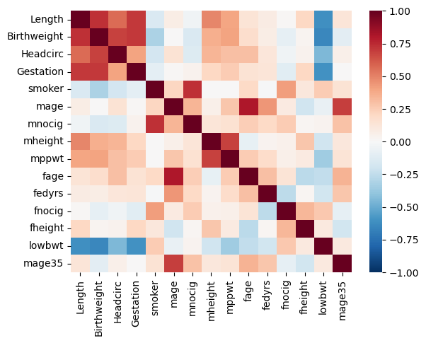
7.3.4 We can also find the correlation between all the variables in our dataframe at once

pearsoncorr = df.corr(method ='pearson')
pearsoncorr

	Length	Birthweight	Headcirc	Gestation	smoker	mage	mnocig	mheight	mppwt	fage	fedyrs	fnocig	fheight	lowbwt	mage35
Length	1.000000	0.726833	0.563172	0.705111	-1.534062e-01	0.075268	-0.039843	0.484992	3.981974e-01	0.137184	0.079485	0.008800	0.208358	-0.609928	0.130502
Birthweight	0.726833	1.000000	0.684616	0.708303	-3.142339e-01	0.000173	-0.152335	0.363055	4.008856e-01	0.175710	0.071045	-0.093136	0.031022	-0.651964	-0.108947
Headcirc	0.563172	0.684616	1.000000	0.404635	-1.828719e-01	0.145842	-0.132988	0.337047	3.028541e-01	0.301151	0.123892	-0.046837	0.041509	-0.446849	0.055386
Gestation	0.705111	0.708303	0.404635	1.000000	-9.474608e-02	0.010778	0.043195	0.210503	2.550824e-01	0.142175	0.130987	-0.113831	0.207597	-0.602935	0.007395
smoker	-0.153406	-0.314234	-0.182872	-0.094746	1.000000e+00	0.212479	0.727218	0.000353	9.808342e-16	0.197501	-0.014891	0.417633	0.110633	0.253012	0.146938
mage	0.075268	0.000173	0.145842	0.010778	2.124788e-01	1.000000	0.340294	0.059956	2.741677e-01	0.806584	0.441683	0.090927	-0.199547	-0.076394	0.692664
mnocig	-0.039843	-0.152335	-0.132988	0.043195	7.272181e-01	0.340294	1.000000	0.126439	1.489446e-01	0.248425	0.198526	0.257307	0.020672	0.035384	0.290574
mheight	0.484992	0.363055	0.337047	0.210503	3.532676e-04	0.059956	0.126439	1.000000	6.806217e-01	-0.079870	0.035297	0.048398	0.274338	-0.198151	0.116002
mppwt	0.398197	0.400886	0.302854	0.255082	9.808342e-16	0.274168	0.148945	0.680622	1.000000e+00	0.255706	0.180374	0.057163	0.092983	-0.353974	0.136853
fage	0.137184	0.175710	0.301151	0.142175	1.975014e-01	0.806584	0.248425	-0.079870	2.557058e-01	1.000000	0.300471	0.135862	-0.269377	-0.245095	0.351405
fedyrs	0.079485	0.071045	0.123892	0.130987	-1.489058e-02	0.441683	0.198526	0.035297	1.803741e-01	0.300471	1.000000	-0.263103	0.017798	-0.191273	0.278682
fnocig	0.008800	-0.093136	-0.046837	-0.113831	4.176330e-01	0.090927	0.257307	0.048398	5.716254e-02	0.135862	-0.263103	1.000000	0.329364	0.266013	-0.088989
fheight	0.208358	0.031022	0.041509	0.207597	1.106327e-01	-0.199547	0.020672	0.274338	9.298347e-02	-0.269377	0.017798	0.329364	1.000000	0.098688	-0.188230
lowbwt	-0.609928	-0.651964	-0.446849	-0.602935	2.530122e-01	-0.076394	0.035384	-0.198151	-3.539738e-01	-0.245095	-0.191273	0.266013	0.098688	1.000000	0.099340
mage35	0.130502	-0.108947	0.055386	0.007395	1.469385e-01	0.692664	0.290574	0.116002	1.368534e-01	0.351405	0.278682	-0.088989	-0.188230	0.099340	1.000000

7.3.5 That isn’t so helpful… we can also make a heatmap to display the data visually

fig, ax = plt.subplots()

sns.heatmap(pearsoncorr,
           cmap='RdBu_r', ax=ax, vmin=-1, vmax=1)

<Axes: >

7.4 Linear Regression

In statistics, linear regression is a linear approach to modeling the relationship between a scalar response and one or more explanatory variables (also known as dependent and independent variables).

https://en.wikipedia.org/wiki/Linear_regression

We have a lot of options for for studying linear regression

7.4.1 Scipy.stats

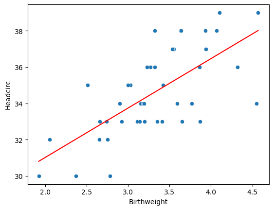
result = scipy.stats.linregress(df['Birthweight'],
                                df['Headcirc'])

print(result)

LinregressResult(slope=2.720563928236349, intercept=25.58239845298082, rvalue=0.6846156184774087, pvalue=5.734797978444235e-07, stderr=0.45798646115832675, intercept_stderr=1.5416553949208147)

A reminder of what the data look like…

fig, ax = plt.subplots()
sns.scatterplot(x=df['Birthweight'], y=df['Headcirc'], ax=ax)
x = np.linspace(df['Birthweight'].min(), df['Birthweight'].max(), 100)
y = result.intercept + result.slope * x
ax.plot(x, y, color='red')

result.slope

2.720563928236349

result.intercept

25.58239845298082

result.rvalue**2

0.46869854506320485

7.4.2 Using sklearn

from sklearn import linear_model

my_model = linear_model.LinearRegression()
results = my_model.fit(df[['Birthweight']], df[['Headcirc']])
print("The linear model is: Y = {:.5} + {:.5}X".format(results.intercept_[0],
                                                       results.coef_[0][0]))

The linear model is: Y = 25.582 + 2.7206X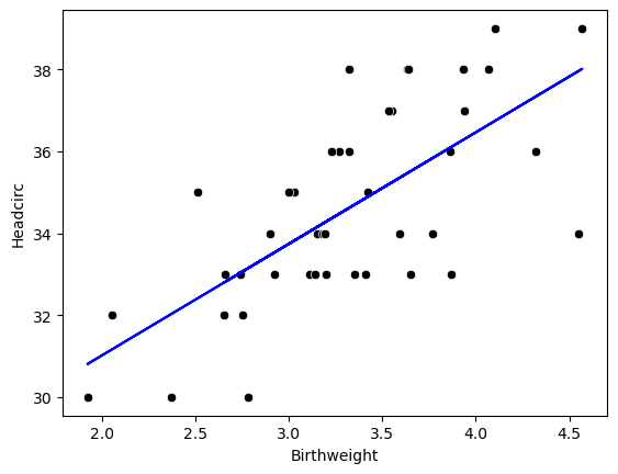

# the results are the same, but the sklearn package has some other features
predictions = results.predict(df[['Birthweight']])

fig, ax = plt.subplots()
# we can add the predicted values to the original plot
ax = sns.scatterplot(x=df['Birthweight'], 
                     y=df['Headcirc'],
                     color="0.0")
ax.plot(df['Birthweight'],
        predictions,
        color="b")

7.5 Hypothesis testing

Null hypothesis 1: The actual intercept is equal to zero
Null hypothesis 2: The actual slope is equal to zero

Using the statsmodels.api package

import statsmodels.api as sm

Set up the model

X = sm.add_constant(df['Birthweight'])
Y = df['Headcirc']
model = sm.OLS(Y, X)  # OLS = ordinary least squares
results = model.fit()
print(results.summary())

                            OLS Regression Results                            
==============================================================================
Dep. Variable:               Headcirc   R-squared:                       0.469
Model:                            OLS   Adj. R-squared:                  0.455
Method:                 Least Squares   F-statistic:                     35.29
Date:                Tue, 16 Jul 2024   Prob (F-statistic):           5.73e-07
Time:                        09:12:12   Log-Likelihood:                -82.574
No. Observations:                  42   AIC:                             169.1
Df Residuals:                      40   BIC:                             172.6
Df Model:                           1                                         
Covariance Type:            nonrobust                                         
===============================================================================
                  coef    std err          t      P>|t|      [0.025      0.975]
-------------------------------------------------------------------------------
const          25.5824      1.542     16.594      0.000      22.467      28.698
Birthweight     2.7206      0.458      5.940      0.000       1.795       3.646
==============================================================================
Omnibus:                        1.089   Durbin-Watson:                   2.132
Prob(Omnibus):                  0.580   Jarque-Bera (JB):                1.007
Skew:                          -0.193   Prob(JB):                        0.604
Kurtosis:                       2.347   Cond. No.                         20.6
==============================================================================

Notes:
[1] Standard Errors assume that the covariance matrix of the errors is correctly specified.

7.5.0.1 The P-value is the answer to the question “how likely is it that we’d get a test statistic t* as extreme as we did if the null hypothesis were true?

Does this output correspond to a one-tailed or two-tailed test?

If we want to test whether the slope is different from 0, we need a two-sided test.

If we want to test a specific direction, we can use a one-sided test. To do this, we need to divide the p-value in the table above in half.

Read more: https://stats.idre.ucla.edu/other/mult-pkg/faq/general/faq-what-are-the-differences-between-one-tailed-and-two-tailed-tests/

print(f'p value of the intercept: {results.pvalues.iloc[0]}, p value of the slope: {results.pvalues.iloc[1]}')

p value of the intercept: 1.5527553380020346e-19, p value of the slope: 5.734797978444454e-07