12 Multiple Linear Regression
TA 11
12.1 Multiple Linear Regression
Multiple Linear Regression Multiple or multivariate linear regression is a case of linear regression with two or more independent variables.
If there are just two independent variables, the estimated regression function is 𝑓(𝑥₁, 𝑥₂) = 𝑏₀ + 𝑏₁𝑥₁ + 𝑏₂𝑥₂. It represents a regression plane in a three-dimensional space. The goal of regression is to determine the values of the weights 𝑏₀, 𝑏₁, and 𝑏₂ such that this plane is as close as possible to the actual responses and yield the minimal SSR.
The case of more than two independent variables is similar, but more general. The estimated regression function is 𝑓(𝑥₁, …, 𝑥ᵣ) = 𝑏₀ + 𝑏₁𝑥₁ + ⋯ +𝑏ᵣ𝑥ᵣ, and there are 𝑟 + 1 weights to be determined when the number of inputs is 𝑟.
https://realpython.com/linear-regression-in-python/#multiple-linear-regression
https://datatofish.com/multiple-linear-regression-python/
Required packages
We will use the birthweight dataset again
| Length | Birthweight | Headcirc | Gestation | smoker | mage | mnocig | mheight | mppwt | fage | fedyrs | fnocig | fheight | lowbwt | mage35 | |
|---|---|---|---|---|---|---|---|---|---|---|---|---|---|---|---|
| 0 | 56 | 4.55 | 34 | 44 | 0 | 20 | 0 | 162 | 57 | 23 | 10 | 35 | 179 | 0 | 0 |
| 1 | 53 | 4.32 | 36 | 40 | 0 | 19 | 0 | 171 | 62 | 19 | 12 | 0 | 183 | 0 | 0 |
| 2 | 58 | 4.10 | 39 | 41 | 0 | 35 | 0 | 172 | 58 | 31 | 16 | 25 | 185 | 0 | 1 |
| 3 | 53 | 4.07 | 38 | 44 | 0 | 20 | 0 | 174 | 68 | 26 | 14 | 25 | 189 | 0 | 0 |
| 4 | 54 | 3.94 | 37 | 42 | 0 | 24 | 0 | 175 | 66 | 30 | 12 | 0 | 184 | 0 | 0 |
12.1.1 Refresher
Last time we examined the relationship between head circumfrence and birthweight
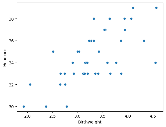
X = sm.add_constant(df.Birthweight)
Y = df.Headcirc
model = sm.OLS(Y, X)
results = model.fit()
print(results.summary())
OLS Regression Results
==============================================================================
Dep. Variable: Headcirc R-squared: 0.469
Model: OLS Adj. R-squared: 0.455
Method: Least Squares F-statistic: 35.29
Date: Mon, 22 Jul 2024 Prob (F-statistic): 5.73e-07
Time: 09:09:45 Log-Likelihood: -82.574
No. Observations: 42 AIC: 169.1
Df Residuals: 40 BIC: 172.6
Df Model: 1
Covariance Type: nonrobust
===============================================================================
coef std err t P>|t| [0.025 0.975]
-------------------------------------------------------------------------------
const 25.5824 1.542 16.594 0.000 22.467 28.698
Birthweight 2.7206 0.458 5.940 0.000 1.795 3.646
==============================================================================
Omnibus: 1.089 Durbin-Watson: 2.132
Prob(Omnibus): 0.580 Jarque-Bera (JB): 1.007
Skew: -0.193 Prob(JB): 0.604
Kurtosis: 2.347 Cond. No. 20.6
==============================================================================
Notes:
[1] Standard Errors assume that the covariance matrix of the errors is correctly specified.12.2 Now, let’s add another predicting variable
What’s the relationship between length and head circumfrence?
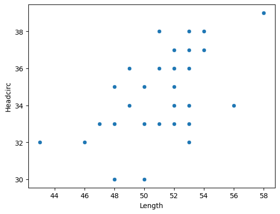
Now we can combine our two ‘predictor’ variables
# using statsmodels
X = sm.add_constant(X)
model = sm.OLS(Y, X).fit()
predictions = model.predict(X)
print_model = model.summary()
print(print_model)
OLS Regression Results
==============================================================================
Dep. Variable: Headcirc R-squared: 0.478
Model: OLS Adj. R-squared: 0.451
Method: Least Squares F-statistic: 17.84
Date: Mon, 22 Jul 2024 Prob (F-statistic): 3.14e-06
Time: 09:10:16 Log-Likelihood: -82.211
No. Observations: 42 AIC: 170.4
Df Residuals: 39 BIC: 175.6
Df Model: 2
Covariance Type: nonrobust
===============================================================================
coef std err t P>|t| [0.025 0.975]
-------------------------------------------------------------------------------
const 21.0794 5.673 3.716 0.001 9.605 32.554
Birthweight 2.3191 0.670 3.464 0.001 0.965 3.673
Length 0.1136 0.138 0.825 0.414 -0.165 0.392
==============================================================================
Omnibus: 1.252 Durbin-Watson: 2.115
Prob(Omnibus): 0.535 Jarque-Bera (JB): 1.122
Skew: -0.224 Prob(JB): 0.571
Kurtosis: 2.337 Cond. No. 1.07e+03
==============================================================================
Notes:
[1] Standard Errors assume that the covariance matrix of the errors is correctly specified.
[2] The condition number is large, 1.07e+03. This might indicate that there are
strong multicollinearity or other numerical problems.# with sklearn
regr = linear_model.LinearRegression()
regr.fit(X, Y)
print('Intercept: ', regr.intercept_)
print('Coefficients: ', regr.coef_)Intercept: 21.079365879118836
Coefficients: [0. 2.319074 0.11363204]So, which package should we use?
In general, scikit-learn is designed for machine-learning, while statsmodels is made for rigorous statistics.
https://medium.com/(hsrinivasan2/linear-regression-in-scikit-learn-vs-statsmodels-568b60792991?)